Getting started
The file fnexamples.py contains examples of Flexible Nets (FNs) stored as Python dictionaries.
The first dictionary in fnexamples.py is net0:
net0 = {
    'name': 'net0',
    'solver': 'glpk',  # Solver to be used
    'places': {        # Places and initial marking
        'p1': 5,       # Initial marking of p1
        'p2': None,    # The initial marking of p2 is not specified
        },
    'm0cons': ["1 <= m0['p2']", "m0['p2'] <= 2"], # Constraints for the
                                                  # initial marking of p2
    'vhandlers': {     # Event handlers
        'v1': [
            {'a': ('p1','v1'), 'b': ('v1','p2')}, # The same amount of tokens
             'a == b'                             # is consumed from p1 and
            ],                                    # produced in p2
        'v2': [
            {'a': ('p2','v2'), 'b': ('v2','p1')},
             'a == b'
            ],
        },
    'obj': {'f': "m['p1']", 'sense': 'max'}, # Objective function
    'options' : {
        'antype': 'un',        # Untimed analysis
        'xlsfile': 'net0.xls', # Results will be stored in this spreadsheet
        'netfile': 'net0.pkl', # The flexible net object with the resulting
                               # variables will be saved in this file
        }
    }
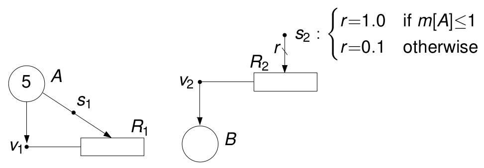
This dictionary specifies a FN with two places and two event handlers. The FN does not have transitions and is therefore untimed. The graphical representation is:

The initial marking of p1 is 5 and the initial marking of p2 can be any value in the interval [1, 2]. Detailed information about the FN formalism can be found in the Bibliography.
The objective function is to maximize the final marking of p1. The solver is GLPK and can be changed by editing the file and setting the value of ‘solver’ to:
'solver': 'cplex',
or
'solver': 'gurobi',
Let’s see how this net can be analyzed from a shell and from the Python interpreter.
Shell script
fnyzer can be executed in a shell as follows:
$ fnyzer fnexamples net0
where fnexample (or fnexample.py) is the file containing the FN specifications and net0 is the name of the dictionary with the FN to be optimized.
The execution of the script produces two files: net0.xls and net0.pkl. net0.xls is a spreadsheet with the values of the variables after the optimization; net0.pkl is a PKL file that stores the FN Python object.
The sheet ‘Untimed’ of the spreadsheet shows the value of the objective function together with the value of the variables. The maximum final marking of p1 is achieved when the initial marking of p2 is 2, i.e. m0[p2]=2, and the event handler v2 is fired in an amount of 2, i.e. dm[(‘v2’, ‘p1’)]=2.
Python interpreter
fnyzer can also be executed from the Python interpreter as shown below:
>>> from fnyzer import optimize
>>> from fnexamples import net0
>>> model, fn = optimize(net0)
This produces the files net0.xls and net0.pkl. The file net0.pkl can be used in a different session to recover the values of the variables:
>>> import pickle
>>> datafile = open("net0.pkl", 'rb')
>>> fn = pickle.load(datafile)
>>> datafile.close()
>>> fn.places
{'p1': <fnyzer.netel.Place object at 0x7fba14aaf588>, 'p2': <fnyzer.netel.Place object at 0x7fba14abc278>}
>>> fn.places['p1']
<fnyzer.netel.Place object at 0x7fba14aaf588>
>>> fn.places['p1'].m
7.0
>>> fn.places['p1'].m0
5.0
>>> fn.varcs[('v2', 'p1')].dm
2.0
optimize() and FNFactory()
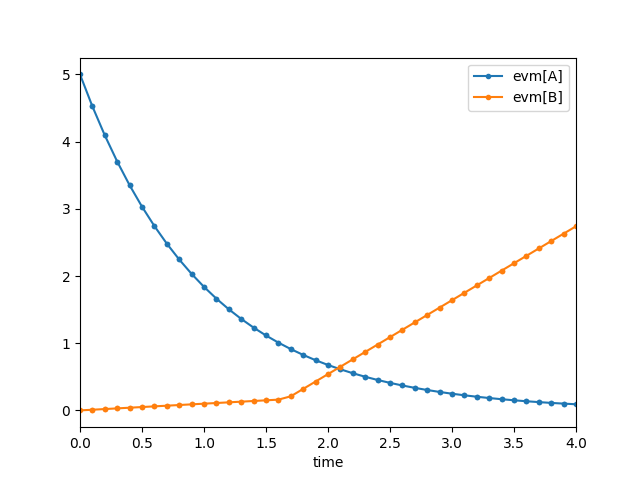
In the following guarded FN, the intensity produced in R2 depends on the marking of A. In particular, the marking of B increases at rate 1.0 when the marking of A is below 1 and at rate 0.1 otherwise.
The specification of this FN can be found in the dictionary ractive of the file fnexamples.py:
ractive = { # Repressor decay activates production
    'name': 'ractive',
    'solver': 'cplex',
    'places': {'A': 5, 'B': 0},
    'trans': {'R1': {'l0': 0, 'a0': 0}, 'R2': {'l0': 0.1, 'a0': 0}},
    'vhandlers': {
        'v1': [{'a': ('A','v1'), 'r': ('R1','v1')}, 'a == r'],
        'v2': [{'b': ('v2','B'), 'r': ('R2','v2')}, 'b == r']
        },
    'regs': {
        'off': ["m['A'] >= 1"],
        'on':  ["m['A'] <= 1"],
        },
    'parts': {'Par': ['off', 'on']},
    'shandlers': {
        's1': [{'a': ('A','s1'), 'r': ('s1','R1')}, 'a == r'],
        's2': [{'r': ('s2','R2')}, {'off': ['r == 0'], 'on': ['r == 1']}]
        },
    'actfplaces': ['A'],
    'exftrans': 'all',
    'actavplaces': ['A'],
    'exavtrans': 'all',
    'obj': {'f': "m['B']", 'sense':'min'},
    'options': {
        'antype' : 'mpc',
        'mpc': {
            'firstinlen': .1,
            'numsteps':   40,
            'maxnumins':  1,
            'flexins': False
            },
        'writevars': {'m': ['A', 'B'], 'l': 'all', 'L': 'all', 'U': 'all'},
        'plotres': True,
        'plotvars': {'evm':['A', 'B']}
        }
}
optimize() and FNFactory() are the main methods provided by fnyzer to optimize a FN specified by a dictionary. While optimize() returns a Pyomo model and a FN object, FNFactory() just returns a FN object. This FN object can be used to call the method optimize():
>>> from fnyzer import FNFactory
>>> from fnexamples import ractive
>>> fnet = FNFactory(ractive)
>>> fnet.optimize()
This produces the files ractive.xls and ractive.pkl and the plot:
The file ractive.pkl can be used in a different session to save the results in a different spreadsheet and to plot the trajectories again:
>>> import pickle
>>> datafile = open("ractive.pkl", 'rb')
>>> fn = pickle.load(datafile)
>>> datafile.close()
>>> fn.writexls("new_ractive.xls")
>>> fn.plotres()